fbprophet

[toc]

1. fbprophet介绍

1.1. fbprophet简介

Prophet（先知）是 Facebook 开源的一个时间序列预测工具，所以叫 fbprophet。Prophet 算法不仅可以处理时间序列存在一些异常值的情况，也可以处理部分缺失值的情形，还能够几乎全自动地预测时间序列未来的走势。从论文上的描述来看，这个 prophet 算法是基于时间序列分解（趋势+季节+节假日）和机器学习的拟合来做的，其中在拟合模型的时候使用了 pyStan 这个开源工具，因此能够在较快的时间内得到需要预测的结果。

Github：https://github.com/facebook/prophet
官方网址：https://github.com/facebook/prophet
论文名字与网址：Forecasting at scale，https://github.com/facebook/prophet

1.2. fbprophet原理

可以先不看原理，看完实例再回来看原理。

• 传统时间序列预测方法缺陷
  • 适用的时序数据过于局限
    例如：最通用的 ARIMA 模型，其要求时序数据是稳定的，或者通过差分化后是稳定的，且在差分运算时提取的是固定周期的信息。
    回忆：automated ARIMA 要求输入的参数是差分的最大阶数、自回归分量和移动平均分量。
  • 缺失值需要填补
  • 模型缺乏灵活性
  • 指导作用较弱

---

• prophet整体框架：Modeling、Forecast Evaluation、Surface Problems 以及 Visually Inspect Forecasts
  
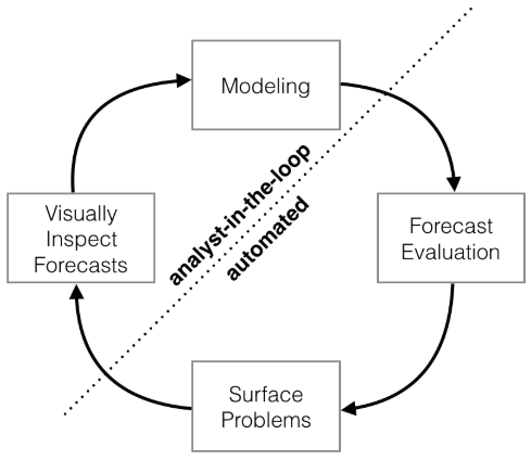
  • Modeling：建立时间序列模型。分析师根据预测问题的背景选择一个合适的模型。
  • Forecast Evaluation：模型评估。根据模型对历史数据进行仿真，在模型的参数不确定的情况下，我们可以进行多种尝试，并根据对应的仿真效果评估哪种模型更适合。
  • Surface Problems：呈现问题。如果尝试了多种参数后，模型的整体表现依然不理想，这个时候可以将误差较大的潜在原因呈现给分析师。
  • Visually Inspect Forecasts：可视化反馈整个预测结果。当问题反馈给分析师后，分析师考虑是否进一步调整和构建模型。

---

• prophet适用场景：
  a. 有至少几个月（最好是一年）的每小时、每天或每周观察的历史数据；
  b. 有多种人类规模级别的较强的季节性趋势：每周的一些天和每年的一些时间；
  c. 有事先知道的以不定期的间隔发生的重要节假日（比如国庆节）；
  d. 缺失的历史数据或较大的异常数据的数量在合理范围内；
  e. 有历史趋势的变化（比如因为产品发布）；
  f. 对于数据中蕴含的非线性增长的趋势都有一个自然极限或饱和状态。

---

• 时间序列分解的三个主要组成部分：growth 增长趋势、seasonality 季节趋势、holidays 节假日
  $$y(t) = g(t) + s(t) + h(t) + \epsilon_t$$
  • $g(t)$：用于拟合时间序列中的分段线性增长或逻辑增长等非周期变化。
  • $s(t)$：周期变化（如：每周/每年的季节性）。
  • $h(t)$：非规律性的节假日效应（用户造成）。
  • $\epsilon_t$：噪声项用来反映未在模型中体现的异常变动，假设服从高斯分布。

---

• $g(t)$ 增长趋势(growth)
  增长趋势是整个模型的核心组件，它表示认为整个时间序列是如何增长的，以及预期未来时间里是如何增长的。这部分为分析师提供了两种模型：Non-linear growth（非线性增长）和 Linear growth（线性增长）。

  
  
  • 1. Non-linear growth（非线性增长）

  非线性增长的公式采用了逻辑回归的模型：${\large g(t) = \frac{C}{1 + e^{-k(t - b)}}}$

  
  其中，$C$ 是承载量，它限定了所能增长的最大值，$k$ 表示增长率，$b$ 为偏移量。（若 $C=1,k=1,m=0$，则是 sigmoid 函数）

  但是，实际的增长模型没有这么简单，所以 Prophet 的作者把这三个参数都换成了随时间变化的函数，即 $C=C(t), k=k(t), m=m(t)$

  而且，在现实的时间序列中，曲线的走势肯定不会一直保持不变，在某些特定的时候或者有着某种潜在的周期曲线会发生变化（变点）。

  
  所以，对于以上问题的解决方法：

  
  （1）将 $C$ 构建成随时间变化的函数：$C(t) = K$ 或者 $C(t) = Mt + K$。（确定 $C(t)$）

  
  （2）在 Prophet 里面设置变点的位置：1.人工指定 n_changepoints；2.算法自动选择。假设已经设置了 $S$ 个变点，并且变点的位置为时间戳 $s_j \ (1 \le j \le S)$。在这些时间戳上，需要知道其增长率的变化，假设有一个向量 $\delta \in \mathbb{R}^S$，其中 $\delta_j$ 表示在时间戳 $s_j$ 上的增长率的变化量。如果一开始的增长率为 $k$，那么在时间戳 $t$ 上的增长率就是 $k + \sum_{j: \ t > s_j}^{}{\delta_j}$。为了简化公式，定义一个指示函数 $a(t) \in {0, 1}^S$ 为 $a_j(t) = \begin{cases}1,&if \ t \ge s_j\0,&otherwise\end{cases}$。那么在时间戳 $t$ 上的增长率就是 $k + a^T\delta$。（确定 $k=k(t)$）

  
  （3）参数 $m$ 确定线段的边界 ${\large \gamma_j = (s_j - m - \sum_{l < j}^{}{\gamma_l})(1 - \frac{k + \sum_{l < j}^{}{\delta_l}}{k + \sum_{l \le j}^{}{\delta_l}})}$（确定 $m=m(t)$）

  
  所以，分段的逻辑回归增长模型就是：${\large g(t) = \frac{C(t)}{1 + e^{-(k + a(t)^t\delta)(t - (m + a(t)^T\gamma))}}}$
  其中，$a(t) = (a_1(t), \dots, a_S(t))^T, \delta = (\delta_1, \dots, \delta_S)^T, \gamma = (\gamma_1, \dots, \gamma_S)^T$
  
  

  • 2. Linear growth（线性增长）

  线性增长采用线性模型：${\large g(t) = (k + a(t)\delta)t + (m + a(t)^T\gamma)}$

  其中，$k$ 表示增长率，$\delta$ 表示增长率的变化量，$m$ 表示偏移参数，$\gamma = (\gamma_1, \dots, \gamma_S)^T, \gamma_j = -s_j\delta_j$ 用于确定线段边界。

---

• $s(t)$ 季节趋势(seasonality)

季节趋势往往呈周期性变化，那么可以通过傅里叶级数表示。傅里叶级数：$$f(x) = a_0 + \sum_{n=1}^{\infty}{(a_n \ cos(nx) + b_n \ sin(nx))}, T = 2\pi$$

Prophet 作者使用傅立叶级数来模拟时间序列的周期性。假设 $P$ 表示时间序列的周期，$P = 365.25$ 表示以年为周期，$P = 7$ 表示以周为周期。它的傅立叶级数的形式都是：$$s(t) = \sum_{n = 1}^{N}{\left( a_n \ cos(\frac{2 \pi n t}{P}) + b_n \ cos(\frac{2 \pi n t}{P}) \right)}$$

就 Prophet 作者经验而言，对于 $P = 365.25$，$N = 10$；对于 $P = 7$，$N = 3$。

傅立叶级数的参数可以形成列向量：$$\beta = (a_1, b_1, \dots, a_N, b_N)^T$$

当 $N = 10$ 时，$$X(t) = \left[cos(\frac{2 \pi (1) t}{365.25}), \dots, sin(\frac{2 \pi (10) t}{365.25}) \right]$$

当 $N = 3$ 时，$$X(t) = \left[cos(\frac{2 \pi (1) t}{7}), \dots, sin(\frac{2 \pi (3) t}{7}) \right]$$

所以，时间序列的季节项就是：${\large s(t) = X(t) \beta, \ \beta \sim N(0, \sigma^2)}$

其中，$\sigma$ = seasonality_prior_scale，$\sigma$ 值越大，表示季节的效应越明显；$\sigma$ 值越小，表示季节的效应越不明显。

seasonality_mode 对应着两种模式： "additive" 加法(默认)和 "multiplicative" 乘法。

$X(t)$ 函数是通过 fourier_series 来构建。

---

• $h(t)$ 节假日(holidays and events)

由于每个节假日对时间序列的影响程度不一样，例如春节，国庆节则是七天的假期，对于劳动节等假期来说则假日较短。因此，不同的节假日可以看成相互独立的模型，并且可以为不同的节假日设置不同的前后窗口值，表示该节假日会影响前后一段时间的时间序列。

对第 $i$ 个节假日来说，$D_i$ 表示该节假日的前后一段时间，$\kappa_i$ 表示该节假日的影响范围，有 $L$ 个节假日。那么时间序列的节假日可以表示为：${\large h(t) = Z(t) \kappa = \sum_\limits{i = 1}^{L}\kappa_i \cdot 1_{ { t \in D_i } } }$

其中，$Z(t) = (1_{ { t \in D_1 } }, \dots, 1_{ { t \in D_L} }), \ \kappa = (\kappa_1, \dots, \kappa_L)^T, \ \kappa \sim N(0, \upsilon^2)$

$\upsilon$ = holidays_prior_scale，默认值是 10，值越大，节假日对模型的影响越大；值越小，节假日对模型的效果越小。

---

• $\epsilon_t$ 噪声

误差项，不需要考虑。。。。。。

---

• fbprophet优点

  1. 大规模、细粒度数据
     能进行大范围预测，并且给出置信区间；数据时间粒度可以很小，支持小时、天、月数据。
  2. 自动处理缺失值数据
     遇到有缺失的数据时其它预测方法需要先进行插值填补预处理，而 fbprophet 可以自己处理缺失值数据。
  3. 更灵活，支持季节、节假日调节
     有些突变点往往是由特别的节假日期引起的，fbprophet 支持输入这些日期以及前后影响的时间窗口，预测的时候自动适这些日期。
  4. 趋势预测 + 趋势分解
     拟合的有两种趋势：线性趋势、逻辑趋势；趋势分解有很多种：Trend、年、周、天趋势、以及节假日效应。
  5. 模型参数易解释
     模型参数很好理解，可以让分析师根据业务经验调节参数来增强某部分假设提高准确率，使模型与业务达到理想的融合。
  6. 拟合速度快
  7. 操作简单
     不仅环境搭建简单，而且只要十几行代码即可完成整个预测过程。

---

• 调参经验

  1. 首先我们去除数据中的异常点（outlier），直接赋值为 None 就可以，因为 Prophet 的设计中可以通过插值处理缺失值，但是对异常值比较敏感。
  2. 选择趋势模型，默认使用分段线性的趋势，但是如果认为模型的趋势是按照 log 函数方式增长的，可设置 growth='logistic' 从而使用分段 log 的增长方式
  3. 设置趋势转折点 changepoint，如果我们知道时间序列的趋势会在某些位置发现转变，可以进行人工设置，比如某一天有新产品上线会影响我们的走势，我们可以将这个时刻设置为转折点。
  4. 设置周期性，模型默认是带有年和星期以及天的周期性，其他月、小时的周期性需要自己根据数据的特征进行设置，或者设置将年和星期等周期关闭。
  5. 设置节假日特征，如果我们的数据存在节假日的突增或者突降，我们可以设置 holiday 参数来进行调节，可以设置不同的 holiday，例如五一一种，国庆一种，影响大小不一样，时间段也不一样。
  6. 此时可以简单的进行作图观察，然后可以根据经验继续调节上述模型参数，同时根据模型是否过拟合以及对什么成分过拟合，我们可以对应调节 seasonality_prior_scale、holidays_prior_scale、changepoint_prior_scale 参数。
  7. 如果预测结果的误差很大，考虑选取的模型是否准确，尝试调整增长率模型 growth 的参数，在必要的情况下也需要调整季节性 seasonality 参数。
  8. 如果在尝试的大多数方法中，某些日期的预测依然存在很大的误差，这就说明历史数据中存在异常值。最好的办法就是找到这些异常值并剔除掉。使用者无需像其他方法那样对剔除的数据进行插值拟合，可以仅保留异常值对应的时间， 并将异常值修改为空值 None，模型在预测时依然可以给出这个时间点对应的预测结果。
  9. 如果对历史数据进行仿真预测时发现，从一个截点到下一个截点误差急剧的增加，这说明在两个截点期间数据的产生过程发生了较大的变化，此时两个截点之间应该增加一个 changepoint ，来对这期间的不同阶段分别建模。
  • a. 如果预测结果的误差很大，考虑选取的模型是否准确，尝试调整增长率模型（growth）的参数，在必要的情况下也需要调整季节性（seasonality）参数。
  • b. 如果在尝试的大多数方法中，某些日期的预测依然存在很大的误差，这就说明历史数据中存在异常值。最好的办法就是找到这些异常值并剔除掉。使用者无需像其他方法那样对剔除的数据进行插值拟合，可以仅保留异常值对应的时间， 并将异常值修改为空值（NA），模型在预测时依然可以给出这个时间点对应的预测结果。
  • c. 如果对历史数据进行仿真预测时发现，从一个截点到下一个截点误差急剧增加，这说明在两个截点期间数据的产生过程发生了较大的变化，此时两个截点之间应该增加一个 changepoint，来对这期间的不同阶段分别建模。

---

fbprophet使用

入门实例

import numpy as np
import pandas as pd
from fbprophet import Prophet

df = pd.read_excel('example_wp_log_peyton_manning.xlsx')
df['y'] = np.log(df['y'])

playoffs = pd.DataFrame({
    'holiday': 'playoff',
    'ds': pd.to_datetime([
        '2008-01-13', '2009-01-03', '2010-01-16',
        '2010-01-24', '2010-02-07', '2011-01-08',
        '2013-01-12', '2014-01-12', '2014-01-19',
        '2014-02-02', '2015-01-11', '2016-01-17',
        '2016-01-24', '2016-02-07']),
    'lower_window': 0,
    'upper_window': 1,
})
superbowls = pd.DataFrame({
    'holiday': 'superbowl',
    'ds': pd.to_datetime(['2010-02-07', '2014-02-02', '2016-02-07']),
    'lower_window': 0,
    'upper_window': 1,
})
holidays = pd.concat((playoffs, superbowls))  # 季后赛和超级碗比赛特别日期
m = Prophet(holidays=holidays)  # 指定节假日参数，其它参数以默认值进行训练

m.fit(df)  # 对过去数据进行训练

future = m.make_future_dataframe(freq='D', periods=365)  # 建立数据预测框架，数据粒度为天，预测步长为一年
forecast = m.predict(future)

m.plot(forecast).show()  # 绘制预测效果图

可以看到 Prophet 遵循 sciket-klearn 模型 API。

fit() 输入的 DataFrame 必须包含两列数据：时间戳 ds 和时间序列的取值 y

在预测效果图中，黑点表示实际值，蓝色表示预测值，浅蓝色表示 yhat_upper 和 yhat_lower，置信区间受到 interval_width 这个参数的影响；当然，从 forecasts 的 keys 中可以看到，还有其他的 _upper 和 _lower，同样也会受到这个参数的影响。

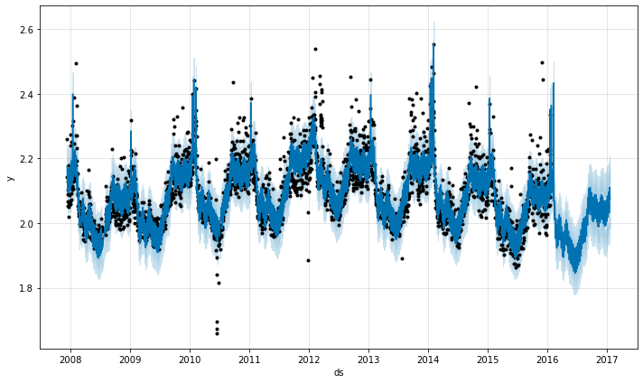
predict() 输出的 DataFrame 包含四列数据：时间戳 ds、时间序列的预测值 yhat、预测值的下界 yhat_lower、预测值的上界 yhat_upper

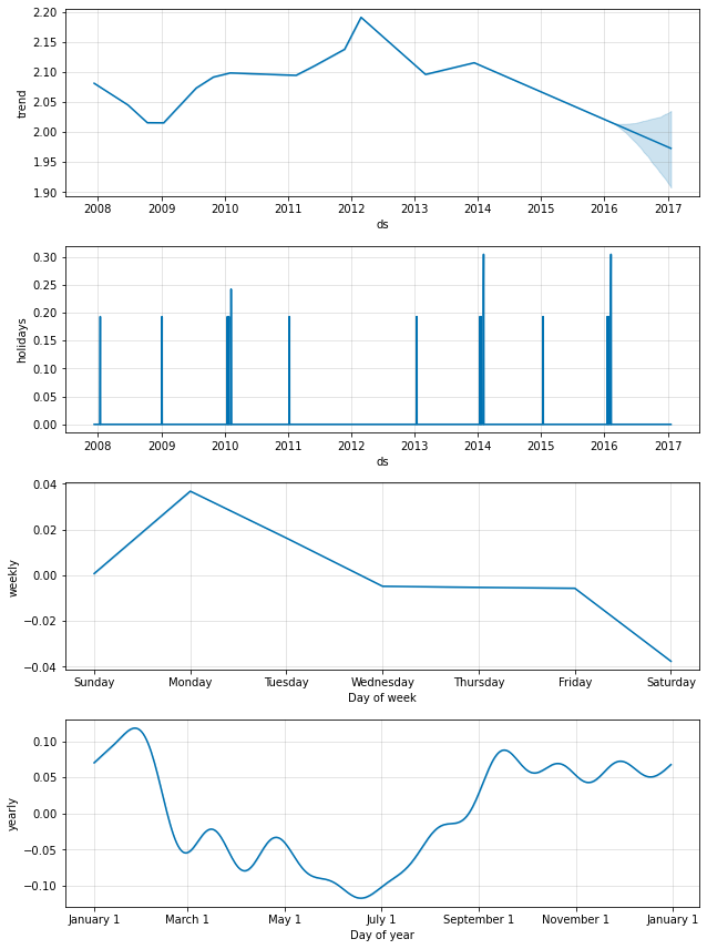
在成分趋势图中，四个图从上至下依次是对增长趋势模型（trend）、节假日模型（holidays）以及季节性模型（weekly 和 yearly）。

所谓成分分析就是指对原理公式中的三大部分模型单独进行分析，成分分析有助于我们考察模型中的各个组件分别对预测结果的影响，通过可视化的展示，我们可以准确判断影响预测效果的具体原因，从而针对性的解决。成分分析是我们提高模型准确性的重要来源。

需要注意的是，如果没有在 holidays 参数里注明具体的节假日信息，模块也不会自动对这一部分进行分析。如果对于上面的结果你觉得有不合理的地方，那么可以根据中参数使用说明更改相应的成分影响，这里应该尽可能的利用你的专业背景知识，以使各部分组成的影响更符合实际。举个例子，如果在每年趋势 yearly 中你认为当前的效果过拟合了，那么就可以调解 seasonality_prior_scale 这个参数，值越小，这里的季节性波动就越小。

Prophet() 类

作用：进行时间序列预测

源代码：

class Prophet(object):
    """Prophet forecaster.

    Parameters
    ----------
    growth: String 'linear' or 'logistic' to specify a linear or logistic
        trend.
    changepoints: List of dates at which to include potential changepoints. If
        not specified, potential changepoints are selected automatically.
    n_changepoints: Number of potential changepoints to include. Not used
        if input `changepoints` is supplied. If `changepoints` is not supplied,
        then n_changepoints potential changepoints are selected uniformly from
        the first `changepoint_range` proportion of the history.
    changepoint_range: Proportion of history in which trend changepoints will
        be estimated. Defaults to 0.8 for the first 80%. Not used if
        `changepoints` is specified.
    Not used if input `changepoints` is supplied.
    yearly_seasonality: Fit yearly seasonality.
        Can be 'auto', True, False, or a number of Fourier terms to generate.
    weekly_seasonality: Fit weekly seasonality.
        Can be 'auto', True, False, or a number of Fourier terms to generate.
    daily_seasonality: Fit daily seasonality.
        Can be 'auto', True, False, or a number of Fourier terms to generate.
    holidays: pd.DataFrame with columns holiday (string) and ds (date type)
        and optionally columns lower_window and upper_window which specify a
        range of days around the date to be included as holidays.
        lower_window=-2 will include 2 days prior to the date as holidays. Also
        optionally can have a column prior_scale specifying the prior scale for
        that holiday.
    seasonality_mode: 'additive' (default) or 'multiplicative'.
    seasonality_prior_scale: Parameter modulating the strength of the
        seasonality model. Larger values allow the model to fit larger seasonal
        fluctuations, smaller values dampen the seasonality. Can be specified
        for individual seasonalities using add_seasonality.
    holidays_prior_scale: Parameter modulating the strength of the holiday
        components model, unless overridden in the holidays input.
    changepoint_prior_scale: Parameter modulating the flexibility of the
        automatic changepoint selection. Large values will allow many
        changepoints, small values will allow few changepoints.
    mcmc_samples: Integer, if greater than 0, will do full Bayesian inference
        with the specified number of MCMC samples. If 0, will do MAP
        estimation.
    interval_width: Float, width of the uncertainty intervals provided
        for the forecast. If mcmc_samples=0, this will be only the uncertainty
        in the trend using the MAP estimate of the extrapolated generative
        model. If mcmc.samples>0, this will be integrated over all model
        parameters, which will include uncertainty in seasonality.
    uncertainty_samples: Number of simulated draws used to estimate
        uncertainty intervals.
    """
    
    def __init__(
            self,
            growth='linear',
            changepoints=None,
            n_changepoints=25,
            changepoint_range=0.8,
            yearly_seasonality='auto',
            weekly_seasonality='auto',
            daily_seasonality='auto',
            holidays=None,
            seasonality_mode='additive',
            seasonality_prior_scale=10.0,
            holidays_prior_scale=10.0,
            changepoint_prior_scale=0.05,
            mcmc_samples=0,
            interval_width=0.80,
            uncertainty_samples=1000,
    ):

• Prophet() 参数说明：
  • growth: 字符串 "linear" 或 "logistic"，表示线性增长趋势或者逻辑增长趋势。
  • changepoints: 日期型向量，指定潜在拐点，如果不指定，将会自动选择潜在拐点。例如：changepoints=["2014-01-01"] 指定 '2014-01-01' 这一天是潜在的 changepoints。
  • n_changepoints: 表示 changepoints 的数量大小，如果 changepoints 指定，该传入参数将不会被使用。如果 changepoints 不指定，将会从输入的历史数据前 $80%$ 中选取 $25$ 个（个数由 n_changepoints 传入参数决定）潜在改变点。
  • changepoint_range: 估计趋势变化点的历史比例。如果指定了 changepoints，则不使用。
  • yearly_seasonality: 指定是否分析数据的年季节性，如果为 True，默认取傅里叶项为 $10$，最后会输出yearly_trend, yearly_upper, yearly_lower 等数据。
  • weekly_seasonality: 指定是否分析数据的周季节性，如果为 True，默认取傅里叶项为 $10$，最后会输出weekly_trend, weekly_upper, weekly_lower 等数据。
  • daily_seasonality: 指定是否分析数据的天季节性，如果为 True，默认取傅里叶项为 $10$，最后会输出daily_trend, daily_upper, daily_lower 等数据。
  • holidays: 传入 DataFrame 格式的数据。这个数据包含有 holiday 列 (string) 和 ds (date类型) 和可选列 lower_window 和 upper_window 来指定该日期的 lower_window 或者 upper_window 范围内都被列为假期。lower_window = -2 将包括前 $2$ 天的日期作为假期。（默认None）
  • seasonality_mode: 季节模型 "additive"(default) or "multiplicative"。
  • seasonality_prior_scale: 调节季节性组件的强度。值越大，模型将适应更强的季节性波动，值越小，越抑制季节性波动。
  • holidays_prior_scale: 调节节假日模型组件的强度。值越大，该节假日对模型的影响越大，值越小，节假日的影响越小。
  • changepoint_prior_scale: 增长趋势模型的灵活度。调节 changepoint 选择的灵活度，值越大选择的 changepoint 越多，使模型对历史数据的拟合程度变强，然而也增加了过拟合的风险。
  • mcmc_samples: mcmc采样，用于获得预测未来的不确定性。若大于 $0$，将做mcmc样本的全贝叶斯推理，如果为 $0$，将做最大后验估计。
  • interval_width: 衡量未来时间内趋势改变的程度。表示预测未来时使用的趋势间隔出现的频率和幅度与历史数据的相似度，值越大越相似。当 mcmc_samples = 0 时，该参数仅用于增长趋势模型的改变程度，当 mcmc_samples > 0 时，该参数也包括了季节性趋势改变的程度。
  • uncertainty_samples: 用于估计不确定性区间的模拟抽取数

make_future_dataframe() 函数

作用：对模型对象和若干时段进行预测，并生成合适的时间数据帧。

源代码：

def make_future_dataframe(self, periods, freq='D', include_history=True):
    """Simulate the trend using the extrapolated generative model.

    Parameters
    ----------
    periods: Int number of periods to forecast forward.
    freq: Any valid frequency for pd.date_range, such as 'D' or 'M'.
    include_history: Boolean to include the historical dates in the data
        frame for predictions.

    Returns
    -------
    pd.Dataframe that extends forward from the end of self.history for the
    requested number of periods.
    """

• make_future_dataframe() 参数说明：
  • periods: 向前预测步数
  • freq: 预测单位，小时为 'H'，天为 'D'，月为 'M'
  • include_history: 是否包含历史数据的预测

简单使用

• STEP
  1. 加载历史数据 df = pd.DataFrame()
  2. 初始化 m = Prophet()
  3. 拟合 m.fit(df)
  4. 加载/生成预测数据 future = pd.DataFrame() / future = m.make_future_dataframe()
  5. 预测 forecast = m.predict(future)
  6. 绘图 m.plot(forecast ) 和 m.plot_components(forecast )

# todo 导入库
import numpy as np
import pandas as pd
import matplotlib.pyplot as plt
from fbprophet import Prophet

# todo 加载数据
data = pd.read_csv('./example_wp_log_peyton_manning.csv')
# todo 查看数据
data.head()

# todo 修改数据列名
df = df.rename(columns={'timestamp': 'ds', 'value': 'y'})

# todo 修改时间数据格式：如果 'timestamp' 是使用 unixtime 来记录的，需要修改成 YYYY-MM-DD hh:mm:ss 的形式
df['ds'] = pd.to_datetime(df['ds'], unit='s')

# todo 时间序列需要进行归一化：
df['y'] = (df['y'] - df['y'].mean()) / (df['y'].std())

# todo 初始化
m = Prophet()

# todo 拟合
m.fit(df)

# todo 预测：生成预测时间数据
future = m.make_future_dataframe(periods=30, freq='M')
"""
periods：需要预测的点数：30个
freq：时间序列的频率：按月来收集的时间序列（'min'分钟）
"""
# todo 展示预测值数据
future.tail()

# todo 预测
forecast = m.predict(future)

# todo 绘制预测图
m.plot(forecast)

# todo 画出时间序列的分量
m.plot_components(forecast)

绘制图：（略）

• STEP
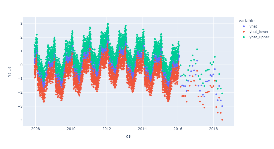
  7. 绘制详细指标图（可交互，结合 plotly）

# todo 导入库
import pandas as pd
import plotly.express as px

# todo 载入数据
df = forecast
# todo 查看数据
df
df.info
df.info()
df.head()
df.describe()

# todo 绘制预测值、预测上下限值
fig = px.scatter(
    data_frame=df, 
    x="ds", 
    y=['yhat', "yhat_lower", "yhat_upper"], 
)

# todo 展示
fig.show()

绘制图：

参数设置

• 变点

m = Prophet(n_changepoints=25)
m = Prophet(changepoint_range=0.8)
m = Prophet(changepoint_prior_scale=0.05)
m = Prophet(changepoints=['2014-01-01'])

# 变点的作图：
from fbprophet.plot import add_changepoints_to_plot
fig = m.plot(forecast)
a = add_changepoints_to_plot(fig.gca(), m, forecast)

• 周期性

m = Prophet(weekly_seasonality=False)
m.add_seasonality(name='monthly', period=30.5, fourier_order=5)
m = Prophet(weekly_seasonality=True)
m.add_seasonality(name='weekly', period=7, fourier_order=3, prior_scale=0.1)

• 节假日

playoffs = pd.DataFrame({
  'holiday': 'playoff',
  'ds': pd.to_datetime(['2008-01-13', '2009-01-03', '2010-01-16',
                        '2010-01-24', '2010-02-07', '2011-01-08',
                        '2013-01-12', '2014-01-12', '2014-01-19',
                        '2014-02-02', '2015-01-11', '2016-01-17',
                        '2016-01-24', '2016-02-07']),
  'lower_window': 0,
  'upper_window': 1,
})
superbowls = pd.DataFrame({
  'holiday': 'superbowl',
  'ds': pd.to_datetime(['2010-02-07', '2014-02-02', '2016-02-07']),
  'lower_window': 0,
  'upper_window': 1,
})
holidays = pd.concat((playoffs, superbowls))

m = Prophet(holidays=holidays, holidays_prior_scale=10.0)

参考

博客园：python 安装fbprophet模块的艰辛历程（安装强推！）
CSDN：python-fbprophet总结（参数说明 + 代码）

这俩差不多：原理 + 使用
标点符：Facebook时间序列预测工具fbprophet（这个内容更多一点）
知乎：Facebook 时间序列预测算法 Prophet 的研究

这俩差不多：例子多
博客园：facebook开源的prophet时间序列预测工具（这个内容更多一点）
CSDN：R+python︱Facebook大规模时序预测『真』神器——Prophet（遍地代码图）

博客园：python时间序列分析（非 Prophet 的时序分析）